the Creative Commons Attribution 3.0 License.
the Creative Commons Attribution 3.0 License.
The bedrock topography of Gries- and Findelengletscher
Nadine Feiger
Matthias Huss
Silvan Leinss
Daniel Farinotti
Knowledge of the ice thickness distribution of glaciers is important for glaciological and hydrological applications. In this contribution, we present two updated bedrock topographies and ice thickness distributions for Gries- and Findelengletscher, Switzerland. The results are based on ground-penetrating radar (GPR) measurements collected in spring 2015 and already-existing data. The GPR data are analysed using ReflexW software and interpolated by using the ice thickness estimation method (ITEM). ITEM calculates the thickness distribution by using principles of ice flow dynamics and characteristics of the glacier surface. We show that using such a technique has a significance advantage compared to a direct interpolation of the measurements, especially for glacier areas that are sparsely covered by GPR data. The uncertainties deriving from both the interpretation of the GPR signal and the spatial interpolation through ITEM are quantified separately, showing that, in our case, GPR signal interpretation is a major source of uncertainty. The results show a total glacier volume of 0.28±0.06 and 1.00±0.34 km3 for Gries- and Findelengletscher, respectively, with corresponding average ice thicknesses of 56.8±12.7 and 56.3±19.6 m.
- Article
(7071 KB) - Full-text XML
-
Supplement
(1475 KB) - BibTeX
- EndNote


Glaciers are essential components in the water cycle, as they can store water over a wide range of timescales (Jansson et al., 2003; Viviroli et al., 2007). The total glacier volume ultimately limits the water amount that can be released by a glacier, and its spatial distribution can have an effect on the timing of said water's release (Gabbi et al., 2012). Knowledge of glacier ice thickness is therefore important not only for a number of glaciological questions but also for questions related to water security (Haeberli and Hölzle, 1995; Immerzeel et al., 2010). In alpine countries such as Switzerland, moreover, hydropower reservoirs are often fed by glacier melt water, thus making estimates of the total glacier volume also relevant from an economic perspective. The increasing demand for renewable energy sources (Kirchner et al., 2012), as well as the long-established role of hydropower as a renewable source (Zimmermann, 2001), additionally fuels the request for precise estimates.
Despite this importance, direct measurements of glacier ice thickness remain sparse around the world (Gaertner-Roer et al., 2014). This is because obtaining such measurements can be laborious and costly, especially for alpine glaciers with rugged topography. Several methods that estimate ice thickness from characteristics of the surface have therefore been presented (Brinkerhoff et al., 2016; Farinotti et al., 2009; Fürst et al., 2017; Linsbauer et al., 2012; Morlighem et al., 2011) (Farinotti et al., 2017; Gaertner-Roer et al., 2014), but direct measurements remain pivotal for both the assessment of their performance and their calibration (Farinotti et al., 2017). It is still under debate, moreover, whether such approaches do indeed outperform a simple interpolation schemes when direct measurements are available.
Ice thickness measurements on glaciers are most often performed with ground-penetrating radar (GPR) Plewes and Hubbard (2001). Depending on the subsurface materials (air, water, ice, snow, sediment) and their specific electromagnetic properties, GPR survey allows detection of interfaces between materials (Daniels, 2007). Since penetration depth of electromagnetic waves generally decreases with higher frequencies, and due to the properties of ice, frequencies between 1 and 1000 MHz are typically used (Yelf, 2007). The choice of the frequency directly relates to the spatial resolution with which individual reflectors can be detected (Van Dam, 2012). On temperate glaciers, signal attenuation can be important and can significantly affect the reliability of measurements (Lapazaran et al., 2016a, b; Martín-Español et al., 2016).
In this contribution, we present two new estimates for the ice thickness distribution and bedrock topography of Gries- and Findelengletscher – two valley glaciers located in catchments exploited for hydropower production in Switzerland (Fig. 1c). The estimates are based on already-existing data acquired between 2009 and 2012, new direct measurements collected during 2015, and the “ice thickness estimation method (ITEM)” (Farinotti et al., 2009). The accuracy of the final product is assessed in a series of sensitivity analysis that combine the uncertainties deriving from both the GPR measurements and the interpolation scheme. The performance of ITEM is additionally compared against a direct interpolation of the measurements.
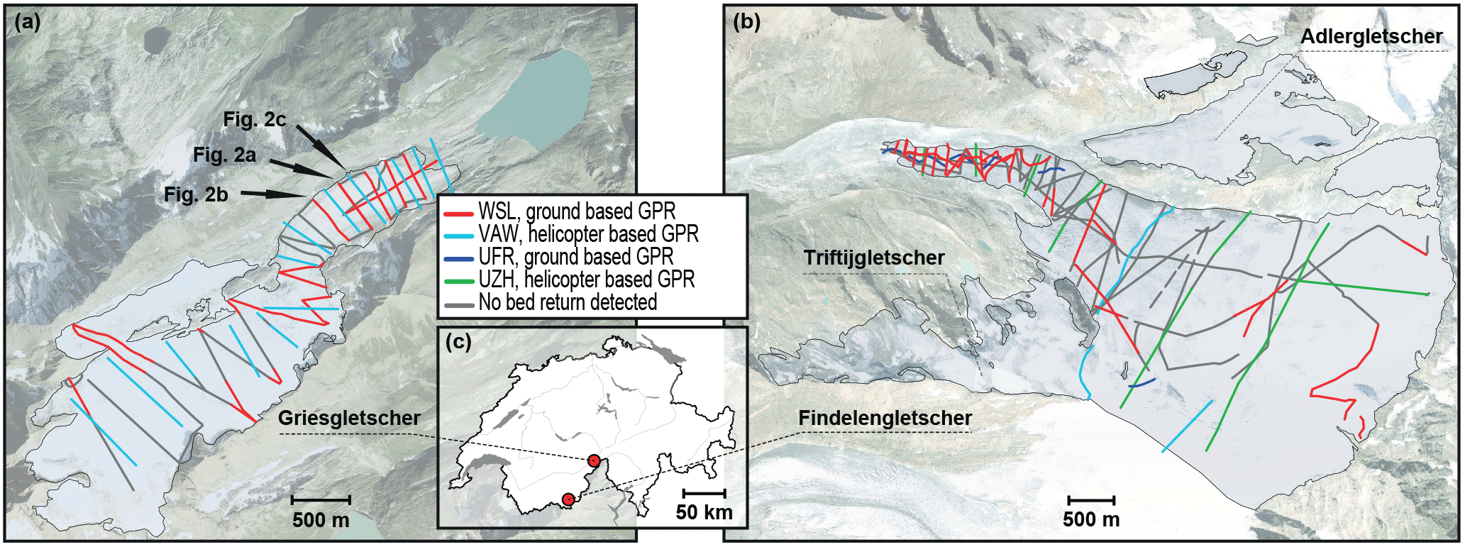
Figure 1 Ground tracks for the GPR measurements collected on (a) Griesgletscher and (b) Findelengeltscher. Radargrams of the profile labelled in (a) are shown in Fig. 2. Abbreviations: WSL – Swiss Federal Institute for Forest, Snow and Landscape Research; VAW – Laboratory of Hydraulics, Hydrology and Glaciology, ETH Zurich; UFR – Department of Geosciences, University of Fribourg; UZH – Department of Geography, University of Zurich. WSL data were collected in 2015, VAW data in 1999 (Gries) and 2008 (Findelen), and UFR and UZH data in 2012. The locations of the glaciers within Switzerland is shown in (c).
Gries- and Findelengletscher (Fig. 1) are two gently sloping valley glaciers with surface areas of ca. 5 and 13 km2, respectively (values refer to 2016). In this work, when we refer to Findelengletscher, we mean the whole glacierized area contained in the corresponding hydrological basin, which notably includes the smaller Triftji- and Adlergletscher (Fig. 1b). The total glacierized area in that basin is ca. 17 km2. The altitude ranges for Griesgletscher and Findelengletscher are 2400–3300 and 2500–3900 m a.s.l., respectively. Both glaciers are part of a mass balance monitoring programme (Huss et al., 2009; Sold et al., 2016).
Past ice thickness measurements on Griesgletscher were performed by the Laboratory of Hydraulics, Hydrology and Glaciology (VAW), ETH Zurich, in 1999. The measurements were performed with the ground-based GPR system described by Bauder et al. (2003). In 2008, measurements on Findelengletscher were recorded by VAW with a helicopter-borne GPR system (Rutishauser et al., 2016) as well as in 2012 by the Department of Geography, University of Zurich (Huss et al., 2014). Additional ground-based GPR measurements were conducted in 2012 by the Department of Geosciences, University of Fribourg (Huss et al., 2014).
The new surveys were conducted on 22 April 2015 on Griesgletscher, and on 26 and 28 February 2015, as well as on 19 March 2015 on Findelengletscher. A MALÅ rough terrain antenna system (http://www.malags.com) with a central frequency of 25 MHz was used. The system was man-towed on skis from the upper area of the glacier to the glacier tongue. The antennas of the system were aligned one after the other along the direction of travel. In addition to the radar data, the geographical position of the traces was recorded with a GARMIN GPSMAP 78s Global Positioning System (GPS) receiver with an estimated position accuracy of ±5 m. The accuracy was estimated by cross-validating the positions provided by the device with the positions of a high-precision GPS receiver (position accuracy better than ±0.05 m) carried in the frame of a separate field campaign. In total, 16 and 25 km of GPR data were collected for Griesgletscher and Findelengletscher, respectively (Table 1). Of these transects, actual bedrock reflections could be detected for 11 km (Griesgletscher) and 13 km (Findelengletscher). The transects are shown in Fig. 1a and b.
For calculating a glacier-wide bedrock topography with the ITEM approach (see next section), further data were required. These included (a) a digital elevation model (DEM) of the glacier surface and (b) a recent glacier outline. For Griesgletscher, a DEM referring to the year 2016 was acquired by the Swiss Federal Office of Topography (swisstopo) in the frame of the GLAMOS (Glacier Monitoring in Switzerland) initiative. For Findelengletscher, the DEM available from GLAMOS for 2016 only covered the elevation below ca. 3300 m a.s.l. For the upper parts of the glacier, the DEM was therefore completed by using two partial DEMs referring to the year 2012 and 2013. These were made available within the frame of the Swiss National Forest Inventory (Ginzler and Hobi, 2015). The completion procedure is expected to introduce only marginal errors, as the surface elevation change for the affected areas is known to be below 0.2 m a−1 (Joerg and Zemp, 2014). The DEMs of both glaciers were resampled to a resolution of 25 m, and glacier outlines referring to 2016 were available.
3.1 GPR data processing
The GPR data were processed with ReflexW software (http://www.sandmeier-geo.de). The best results in terms of bedrock-reflection visibility were obtained applying the following processing sequence:
-
Moving the start time: the time-zero correction was moved to the first detectable break in the radargrams to match start time with surface position.
-
Interpolation to equidistant traces: the original data showed heterogeneous spacing between traces caused by varying survey speed. This processing step ensured a constant spacing, chosen to be 0.1 m.
-
Frequency bandpass filter: to dewow the data, a trapezoidal frequency bandpass filter was applied. The frequency range from the lower and upper cut-off was chosen to be 6 and 32 MHz, respectively.
-
Background removal: to remove persistent noise within individual radargrams, a background-removal filter was applied. The filter basically subtracts the average signal of all traces.
-
Divergence compensation: a time-proportional divergence compensation gain was applied in order to compensate for the geometrical divergence losses in signal amplitude with depth. The according scaling value was set to 0.01.
-
Frequency-wave-number (fk) migration: in many profiles, bedrock reflections towards the margins of the glacier were obscured by straight-line events crossing the records with a uniform apparent dip. Partial removal of these events, originating from air wave reflections at the side walls of the glacier, was achieved by applying a fk filter Yilmaz (2001).
After application of the processing steps above, bedrock reflections were manually picked on the radargrams. When more than one reflector layer was present in the same radargram, all layers were picked in the first instance. Data segments without any visible reflector were discarded. The signal travel time was converted into ice thickness, under the assumption of a uniform wave velocity of 0.167 m ns−1 (Robin et al., 1969). Velocity changes in the firn layer were neglected in the light of its small thickness in the surveyed areas. Note that Griesgletscher has presently a very reduced firn cover Glaciological Reports (1881), whilst the profiles on Findelengletscher are mostly located in the ablation zone (Fig. 1b).
3.2 Data selection
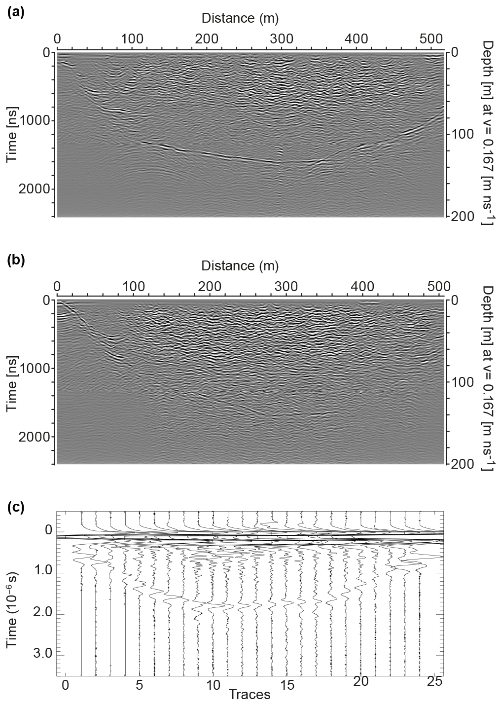
Figure 2 Examples of ground-based GPR radargrams available for Griesgletscher. Panels (a) and (b) give a visual impression of a good- and a poor-quality profile collected at a frequency of 25 MHz during 2015. Panel (c) shows an example for GPR radargrams collected at a frequency between 1 and 8 MHz in 1999 by VAW. The locations of the profiles are shown in Fig. 1a.
Table 1Acquired and utilized GPR measurements for Gries- and Findelengletscher. The year in which the data were collected and the collecting institute are given. Institute abbreviations are given in the caption of Fig. 1.
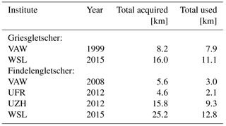
Figure 2a and b show two ground-based GPR profiles as an example for radargrams with good and poor quality, respectively. In the case of ambiguity, the correct reflection layer for each profile was identified by comparing profiles at their crossover points. The most plausible set of reflector layers for each glacier was identified by maximizing the consistency at such points. Already-existing ground-based and helicopter-borne GPR data were included in the consistency analysis. The final dataset was optically tested for consistency through 3-D visualization. The resulting final selection of profiles is shown in Fig. 1 and summarized in Table 1.
3.3 Glacier-wide estimates
To obtain a glacier-wide bedrock topography, the GPR dataset was interpolated by using the ITEM approach (Farinotti et al., 2009). ITEM calculates the ice thickness distribution by using principles of ice flow dynamics along selected flow lines. The mass turnover along these flow lines is calculated by integrating the glacier surface mass balance distribution. The so-derived ice volume flux is then converted into ice thickness by using Glen`s flow law (Glen, 1955). Uncertainties deriving from basal sliding and the chosen flow parameters are accounted for in a correction factor C (see Eq. 7 by Farinotti et al., 2009) that is adjusted to individually match the available GPR transects. To ensure a smooth transition of C between the transects, and to interpolate the ice thickness between individual flow lines, an interpolation scheme based on the minimum-curvature method (Briggs, 1974) was used. Finally, a glacier-wide bedrock topography was calculated by subtracting the generated ice thickness distribution from the given glacier surface (DEM).
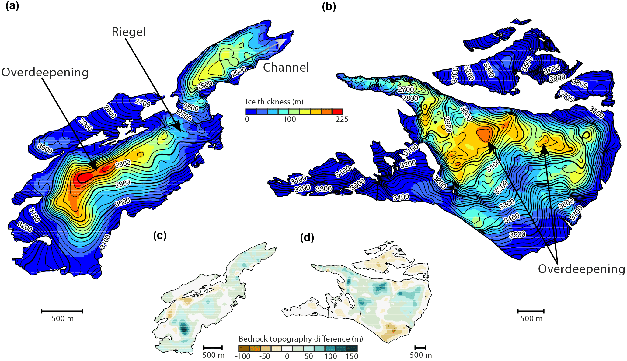
Figure 3 Ice thickness distribution for (a) Griesgletscher and (b) Findelengletscher. The contour lines refer to the bedrock topography and have an interval of 20 m. A comparison with previous estimates (Farinotti et al., 2012) is shown in (e) and (d).
Figure 3a and b show the ice thickness distribution derived for Gries- and Findelengletscher, as well as the resulting bedrock topography. Spatially distributed estimates for the accuracy of the results are shown in Fig. 4. The total ice volume (glacier area) for Gries- and Findelengletscher is 0.28±0.06 km3 (4.9 km2) and 1.00±0.34 km3 (17.4 km2), respectively. Note, again, that when referring to Findelengletscher, we are referring to the whole glacierized area in its hydrological basin, thus including Adlergletscher and Triftjigletscher. The above values correspond to an average ice thickness of 56.8±12.7 m for Griesgletscher and 56.3±19.6 m for Findelengletscher. The thickest ice for Griesgletscher is found in the upper, relatively flat part around 3000 m a.s.l. with an ice thickness of ca. 220 m. For Findelengletscher, the maximal ice thickness is ca. 185 m, also located in the upper, relatively flat part at about 3300 m a.s.l.
The results for Findelengletscher (Fig. 3b) show some marked overdeepenings on the orographic left- and right-hand side of the glacier. The bedrock topography of Griesgletscher shows a typical valley shape with a bedrock riegel between 2700 and 2900 m a.s.l., and an overdeepening behind this.
When the computed bedrock topographies are compared to previous estimates (Farinotti et al., 2012; Huss et al., 2014), local discrepancies between −75 and 141 m emerge for Griesgletscher, and between −94 and 107 m for Findelengletscher. These large deviations are found for locations far away from measured profiles, which is indicative of the choice of the procedure by which measurements are interpolated to play an important role (see also next section). The magnitude of the deviations also increases with increasing ice thickness.
5.1 Accuracy of GPR measurements
Several factors limit the accuracy of GPR measurements, including (1) uncertainties in the exact position of the transmitter and the receiver during the data collection process; (2) variations in the geometrical setting of the radar antennas when travelling; (3) uncertainties in the assumed wave velocity for converting signal travel time to depth; (4) differences in the wave velocity for firn, snow, and ice; (5) choice of processing steps and parameters during the data post-processing; (6) uncertainties in the interpretation of the post-processed radargrams; and (7) the accuracy with which a detected reflector can be picked manually. Whilst points (1) and (2) are likely to lead to minor deviations in the measurements, factors (3) and (5) could cause systematic deviation. In our case, (4) was negligible due to the shallow firn layer. The main source of uncertainty was in (6) and (7), which is related to the quality of the radargrams and the often weak signal return.
To quantify the uncertainty introduced by the GPR measurements, the following analysis was performed:
- a.
For each GPR profile collected in 2015, a minimum and a maximum ice thickness was selected. This selection was based on a different interpretation of the GPR return signal, whereby the minimum (maximum) ice thickness was defined from the highest (deepest) possible bedrock conceivable with the data at hand. The uncertainty range results as the difference between these two choices and reflects the uncertainty in the interpretation of the radargrams.
- b.
For GPR data collected before 2015, the uncertainty was estimated based on the corresponding reports (Huss et al., 2014). In the case of Griesgletscher, radargrams had a high and homogeneous quality, with an estimated uncertainty of the order of ±5 m. For Findelengletscher, the reported quality was lower, and a conservative range of ±15 % was assumed. In this case, expressing the range as a percentage allowed the fact that deeper profiles had larger uncertainties to be taken into account.
- c.
The GPR profiles where adjusted by adding or subtracting half of the uncertainty ranges estimated in (a) and (b). This resulted in two different sets of adjusted profiles, which where then used to compute two different bedrock topographies with the same procedure as for the original profiles (cf. Sect. 3.3). The difference between these bedrock topographies was used as a metric to quantify the uncertainty deriving from the GPR data (Fig. 4a+b).

Figure 4 Spatially distributed estimate of overall uncertainty for (a) Gries- and (b) Findelengletscher. The estimates were generated by combing the uncertainty deriving from the GPR measurements (c+e) and the uncertainty introduced by the ITEM approach (d, f) in quadrature.
5.2 Accuracy of the ITEM approach
The uncertainty of the calculated ice thickness distribution is caused not only by the uncertainty of the direct measurements alone but also by the uncertainty introduced by the application of the ITEM approach. To quantify the latter, we performed a resampling experiment in which we randomly omitted a given number of GPR profiles during the calculations. For each of these resampling steps, a glacier-wide bedrock topography was computed, and the omitted profiles were used for cross-validating the results. The procedure was repeated 500 times for randomly selected combinations of GPR profiles. The ensemble of resulting cross-validation points was used to estimate a function relating (i) the local deviation between measured and estimated ice thickness to (ii) the distance of the closest GPR measurement (Fig. 5). This function was chosen to be linear and was fitted through robust regression of all cross-validation points (blue lines in Fig. 5). The function was then used to generate a spatially distributed uncertainty estimate (Fig. 4d, f). As expected, the uncertainty in the local ice thickness increased with the distance to the closest GPR point (Fig. 5). On average, the uncertainty increased by 4.8 % for every kilometre of distance for both Gries- and Findelengletscher.
To put the uncertainty caused by the ITEM approach into context, we performed a similar resampling experiment for the case in which the available GPR measurements are interpolated directly. For that, the same 500 random profile combinations were used and interpolated by using a minimum-curvature method (Briggs, 1974). For the interpolation, the information of “zero ice thickness at the glacier margin” was included. The minimum-curvature method was preferred over the sometimes-applied ANUDEM interpolation (Hutchinson, 1989), as – contrary to ANUDEM – it does not introduce geometrical features that are not present in the original data (Briggs, 1974). The function relating the deviation between measured and estimated ice thickness to the distance of the closest GPR measurement is again shown in Fig. 5. The fitted linear function reveals that the uncertainty increased by 8.5 % per kilometre on both glaciers. This is almost twice as much as for the case in which ITEM is applied, and it indicates the added value of using an approach based on glaciological principles. The added value is particularly relevant in cases where only sparse GPR measurement are available, i.e. in cases for which the distance between individual GPR transects is large.
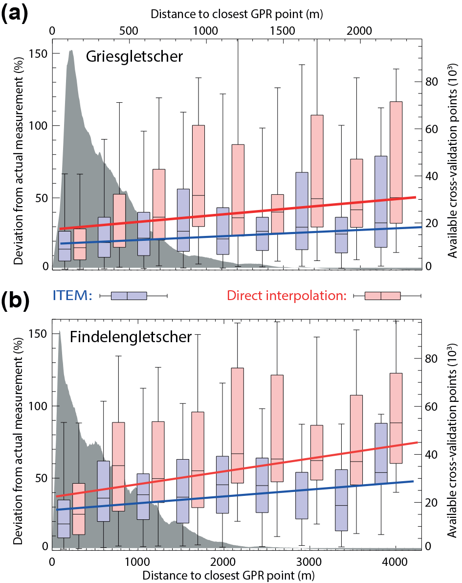
Figure 5 Relation between local bedrock uncertainty and distance to the closest GPR point (box plots, left ordinate), and number of cross-validation points available for a given distance (grey shading, right ordinate). The fitted linear function was derived by robust regression of all bins that have at least 20 cross-validation points. Box plots and fits are shown for the situation in which the bedrock is derived from ITEM (blue colours) and from direct interpolation of the GPR measurements (red colours). Box plots show the median (horizontal line), the interquartile range (box), and an empirical 95 % confidence interval (whiskers).
5.3 Combined accuracy of the results
The final accuracy estimate for the glacier-wide ice thickness was obtained by combining in quadrature the two distributed accuracy estimates discussed above (accuracy of GPR measurements and accuracy of the ITEM approach). Note that the combination in quadrature requires the assumption of independence between the two uncertainty sources. This seems reasonable since neither is the procedure used within ITEM changing for different numerical values of the GPR measurements, nor are the GPR measurements influenced by the ITEM procedure. The resulting uncertainty for the glacier-wide ice thickness is shown in Fig. 4a and b. The mean uncertainty was calculated to be ± 12.7 m for Griesgletscher and ± 19.6 m for Findelengletscher. The combined results show that, in our case, the largest uncertainty is due to the difficulty in interpreting the GPR measurements. Compared to that, the uncertainty introduced through ITEM is minor for the largest part of the glacier.
On Griesgletscher, an overdeepening is found behind a bedrock riegel in the upper part of the glacier. With glacier retreat, water might be dammed behind this riegel and a lake could be forming. Further, a channel is visible in the bedrock on the left-hand side of the glacier tongue. Independent indications for the existence of such a channel were recently obtained from dye-tracing experiments conducted in the frame of a different project (M. Selenius, personal communication, 2017). It seems therefore very likely that most of the glacier runoff occurs through this channel. This may in turn have an impact on the existing artificial lake and the related hydropower station as the channel is indicative for preferential sediment evacuation occurring along this axis.
On Findelengletscher, a prominent overdeepening is visible at an elevation of ca. 3200 m a.s.l. (cf. Fig. 3b). The comparison with previous estimates and the presented uncertainty assessment, however, clearly indicates that significant uncertainty is affecting this area. This is because only few measurements are available in that region. The lack of direct measurements also affects other areas, most notably Adlergletscher and Triftjigletscher. Although the uncertainty is well reflected by the function taking into account the distance to the closest GPR measurement (Fig. 5), additional GPR measurements would be necessary to improve the results.
The difficulty in correctly interpreting the acquired radargrams is a major source of uncertainty in our analysis. To increase the quality of the radargrams, the orientation of the GPR antennas should be along the glacier flow, instead of across the glacier flow (Langhammer et al., 2017). Such an orientation, however, was not practicable in the field with the available MALÅ system.
In summary, we provided an updated glacier-wide bedrock topography for Gries- and Findelengletscher further improving the data basis for glaciological and hydrological applications in the region. Our results are based on 24 km of new ground-based GPR measurements, a series of 22 km of already-existing helicopter- and ground-based GPR measurements, and the ITEM approach (Farinotti et al., 2009). Our accuracy assessment, which combined uncertainties deriving from both GPR measurements and ITEM approach, indicates a mean point-uncertainty of ±12.7 m for Griesgletscher and ±19.6 m for Findelengletscher. The estimated total ice volume is 0.28±0.06 km3 for Griesgletscher and 1.00±0.34 km3 for Findelengletscher. Additionally, we showed that using the ITEM approach has a significant advantage as compared to a direct interpolation of the GPR measurements and that the interpretation of the GPR signal can be a major source of uncertainty.
The code used during the analyses is available upon request. The results of this study are available as an electronic supplement to this article.
The supplement related to this article is available online at: https://doi.org/10.5194/gh-73-1-2018-supplement.
DF, MH, SL, and LS collected data in the filed. NF analysed the GPR data with support from DF. NF and DF performed the ITEM simulations. NF wrote the article and prepared all figures with contributions from DF and MH.
The authors declare that they have no conflict of interest.
We thank all members of the field campaigns on Griesgletscher
and Findelengletscher, particularly including Julia Schmale, Anita
Bianchi, and Ladina Glaus. We are indebted to Gwendolyn Leysinger Vieli and
Andreas Vieli, from whom we borrowed the GPR system during the 2015 GPR campaign.
Christian Ginzler provided the surface DEMs associated with the Swiss National
Forest Inventory. The UZH GPR measurements were collected in the frame of
the “GLAXPO (Glacier Laserscanning Experiment Oberwallis)” project.
The comments of two anonymous reviewers helped to improve the manuscript.
Edited by: Martin Hoelzle
Reviewed by: two anonymous referees
Bauder, A., Funk, M., and Gudmundsson, G. H.: The ice thickness distribution of Unteraargletscher (Switzerland), Ann. Glaciol., 37, 331–336, https://doi.org/10.3189/172756403781815852, 2003. a
Briggs, I. C.: Machine contouring using minimum curvature, Geophysics, 39, 39–48, https://doi.org/10.1190/1.1440410, 1974. a, b, c
Brinkerhoff, D. J., Aschwanden, A., and Truffer, M.: Bayesian inference of subglacial topography using mass conservation, Front. Earth Sci., 4, 1–15, https://doi.org/10.3389/feart.2016.00008, 2016. a
Daniels, D.: Ground penetrating radar (2nd ecition), The Institution of Engineering and Technology, London, 2007. a
Farinotti, D., Huss, M., Bauder, A., Funk, M., and Truffer, M.: A method to estimate ice volume and ice thickness distribution of alpine glaciers, J. Glaciol., 55, 422–430, https://doi.org/10.3189/002214309788816759, 2009. a, b, c, d, e
Farinotti, D., Usselmann, S., Huss, M., Bauder, A., and Funk, M.: Runoff evolution in the Swiss Alps: Projections for selected high-alpine catchments based on ENSEMBLES scenarios, Hydrol. Process., 26, 1909–1924, https://doi.org/10.1002/hyp.8276, 2012. a, b
Farinotti, D., Brinkerhoff, D. J., Clarke, G. K. C., Fürst, J. J., Frey, H., Gantayat, P., Gillet-Chaulet, F., Girard, C., Huss, M., Leclercq, P. W., Linsbauer, A., Machguth, H., Martin, C., Maussion, F., Morlighem, M., Mosbeux, C., Pandit, A., Portmann, A., Rabatel, A., Ramsankaran, R., Reerink, T. J., Sanchez, O., Stentoft, P. A., Singh Kumari, S., van Pelt, W. J. J., Anderson, B., Benham, T., Binder, D., Dowdeswell, J. A., Fischer, A., Helfricht, K., Kutuzov, S., Lavrentiev, I., McNabb, R., Gudmundsson, G. H., Li, H., and Andreassen, L. M.: How accurate are estimates of glacier ice thickness? Results from ITMIX, the Ice Thickness Models Intercomparison eXperiment, The Cryosphere, 11, 949–970, https://doi.org/10.5194/tc-11-949-2017, 2017. a, b
Fürst, J. J., Gillet-Chaulet, F., Benham, T. J., Dowdeswell, J. A., Grabiec, M., Navarro, F., Pettersson, R., Moholdt, G., Nuth, C., Sass, B., Aas, K., Fettweis, X., Lang, C., Seehaus, T., and Braun, M.: Application of a two-step approach for mapping ice thickness to various glacier types on Svalbard, The Cryosphere, 11, 2003–2032, https://doi.org/10.5194/tc-11-2003-2017, 2017. a
Gabbi, J., Farinotti, D., Bauder, A., and Maurer, H.: Ice volume distribution and implications on runoff projections in a glacierized catchment, Hydrol. Earth Syst. Sci., 16, 4543–4556, https://doi.org/10.5194/hess-16-4543-2012, 2012. a
Gaertner-Roer, I., Naegeli, K., Huss, M., Knecht, T., Machguth, H., and Zemp, M.: A database of worldwide glacier thickness observations, Global Planet. Change, 122, 330–344, https://doi.org/10.1016/j.gloplacha.2014.09.003, 2014. a, b
Ginzler, C. and Hobi, M. L.: Countrywide Stereo-Image Matching for Updating Digital Surface Models in the Framework of the Swiss National Forest Inventory, Remote Sens., 7, 4343–4370, https://doi.org/10.3390/rs70404343, 2015. a
Glaciological Reports: The Swiss Glaciers, 1880–2015, Tech. Rep. 1–136, Yearbooks of the Cryospheric Commission of the Swiss Academy of Sciences (SCNAT), published since 1964 by Laboratory of Hydraulics, Hydrology and Glaciology (VAW) of ETH Zürich, 1881–2017. a
Glen, J.: The creep of polycrystalline ice, P. Roy. Soc. Lond. A Mat., 228, 519–538, https://doi.org/10.1098/rspa.1955.0066, 1955. a
Haeberli, W. and Hölzle, M.: Application of inventory data for estimating characteristics of and regional climate-change effects on mountain glaciers: a pilot study with the European Alps, Ann. Glaciol., 21, 206–212, 1995. a
Huss, M., Bauder, A., and Funk, M.: Homogenization of long-term mass balance time series, Ann. Geophys., 50, 198–206, https://doi.org/10.3189/172756409787769627, 2009. a
Huss, M., Zemp, M., Joerg, P. C., and Salzmann, N.: High uncertainty in 21st century runoff projections from glacierized basins, J. Hydrol., 510, 35–48, https://doi.org/10.1016/j.jhydrol.2013.12.017, 2014. a, b, c, d
Hutchinson, M. F.: A new procedure for gridding elevation and stream line data with automatic removal of spurious pits, J. Hydrol., 106, 211–232, https://doi.org/10.1016/0022-1694(89)90073-5, 1989. a
Immerzeel, W., van Beek, L., and Bierkens, M.: Climate change will affect the Asian water towers, Science, 328, 1382–1385, https://doi.org/10.1126/science.1183188, 2010. a
Jansson, P., Hock, R., and Schneider, T.: The concept of glacier storage: a review, J. Hydrol., 282, 116–129, 2003. a
Joerg, P. C. and Zemp, M.: Evaluating Volumetric Glacier Change Methods Using Airborne Laser Scanning Data, Geogr. Ann. A, 96, 135–145, https://doi.org/10.1111/geoa.12036, 2014. a
Kirchner, A., Bredow, D., Ess, F., Grebel, T., Hofer, P., Kemmler, A., and Struwe, J.: Die Energieperspektiven für die Schweiz bis 2050, Bundesamt für Energie (BFE), Bern, Switzerland, 2012. a
Langhammer, L., Rabenstein, L., Bauder, A., and Maurer, H.: Ground-penetrating radar antenna orientation effects on temperate mountain glaciers, Geophysics, 82, H15–H24, https://doi.org/10.1190/geo2016-0341.1, 2017. a
Lapazaran, J., Otero, J., Martín-Español, A., and Navarro, F.: On the errors involved in ice-thickness estimates I: ground-penetrating radar measurement errors, J. Glaciol., 62, 1008–1020, 2016a. a
Lapazaran, J., Otero, J., Martín-Español, A., and Navarro, F.: On the errors involved in ice-thickness estimates II: errors in digital elevation models of ice thickness, J. Glaciol., 62, 1021–1029, https://doi.org/10.1017/jog.2016.94, 2016b. a
Linsbauer, A., Paul, F., and Haeberli, W.: Modeling glacier thickness distribution and bed topography over entire mountain ranges with GlabTop: Application of a fast and robust approach., J. Geophys. Res., 117, F03007, https://doi.org/10.1029/2011JF002313, 2012. a
Martín-Español, A., Lapazaran, J., Otero, J., and Navarro, F.: On the errors involved in ice-thickness estimates III: error in volume, J. Glaciol., 62, 1030–1036, https://doi.org/10.1017/jog.2016.95, 2016. a
Morlighem, M., Rignot, E., Seroussi, H., Larour, E., Dhia, H. B., and Aubry, D.: A mass conservation approach for mapping glacier ice thickness, Geophys. Res. Lett., 38, L19503, https://doi.org/10.1029/2011GL048659, 2011. a
Plewes, L. and Hubbard, B.: A review of the use of radio-echo sounding in glaciology, Prog. Phys. Geog., 25, 203–236, https://doi.org/10.1177/030913330102500203, 2001. a
Robin, G. D. Q., Evans, S., and Bailey, J. T.: Interpretation of radio echo sounding in polar ice sheets, P. Roy. Soc. Lond. A Mat., 265, 437–505, https://doi.org/10.1098/rsta.1969.0063, 1969. a
Rutishauser, A., Maurer, H., and Bauder, A.: Helicopter-borne ground-penetrating radar investigations on temperate alpine glaciers: A comparison of different systems and their abilities for bedrock mapping, Geophysics, 81, WA119–WA129, https://doi.org/10.1190/GEO2015-0144.1, 2016. a
Sold, L., Huss, M., Machguth, H., Joerg, P. C., Vieli, G. L., Linsbauer, A., Salzmann, N., Zemp, M., and Hoelzle, M.: Mass Balance Re-analysis of Findelengletscher, Switzerland, Benefits of Extensive Snow Accumulatin Measurements, Front. Earth Sci., 4, https://doi.org/10.3389/feart.2016.00018, 2016. a
Van Dam, R. L.: Landform characterization using geophysics Recent advances, applications, and emerging tools, Geomorphology, 137, 57–73, https://doi.org/10.1016/j.geomorph.2010.09.005, 2012. a
Viviroli, D., Dürr, H., Messerli, B., and Meybeck, M.: Mountains of the world, water towers for humanity: Typology, mapping, and global significance, Water Resour. Res., 43, W07447, https://doi.org/10.1029/2006WR005653, 2007. a
Yelf, R. J.: Application of ground penetrating radar to civil and geotechnical engineering, Electromagnetic Phenomena, 7, 102–117, https://doi.org/10.1109/IWAGPR.2013.6601528, 2007. a
Yilmaz, O.: Seismic Data Analysis: Processing, Inversion, and Interpretation of Seismic Data, vol. II, Society of Exploration Geophysicists, ISBN-13: 978-1-56080-099-6, Istanbul, Turkey, 2001. a
Zimmermann, M.: Energy situation and policy in Switzerland, International Journal of Ambient Energy, 22, 29–34, https://doi.org/10.1080/01430750.2001.9675384, 2001. a
ice thickness estimation method (ITEM). The results show a total glacier volume of 0.28 ± 0.06 and 1.00 ± 0.34 km3 for Gries- and Findelengletscher, respectively, with corresponding average ice thicknesses of 56.8 ± 12.7 and 56.3 ± 19.6 m.